Turtle tiles part 2: Properties of coloured Kagome lattices

This is a direct sequel to the last post on the Turtle Tile. Please read that first to make sense of this post.

In accounts of the discovery of the Hat aperiodic monotile such as [1], one of the first clues to the structure of its tilings was the fact that reflected Hat tiles seemed to always be placed sparsely yet evenly within the tiling.

Figure 0: A patch of Hat tiles. Reflected tiles are orange, unreflected tiles are blue.

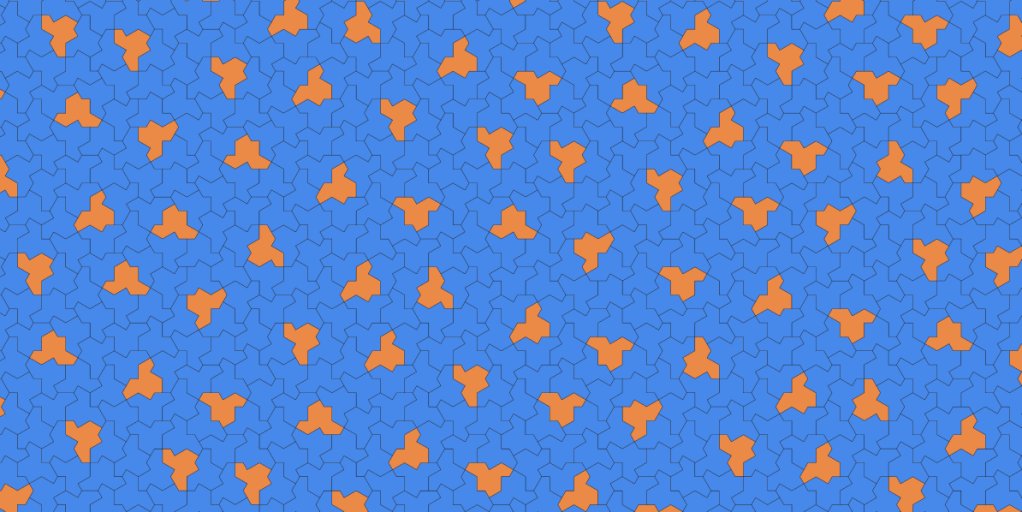
This observation eventually led to the discovery of the metatiles in [2] and their substitutions. Those substitutions imply that there are just under seven unreflected Hat tiles for every reflected Hat tile. This explains the sparseness of reflected tiles, but the ‘evenness’ can only be seen after careful consideration of metatile arrangements.

The nature of the reflected tile placement can be directly addressed in Turtle tilings. In this post, I prove that, in a sense, reflected Turtle tiles are placed ‘as evenly as possible’ in the tiling. This proof is convoluted, so we will also discuss how this ‘evenness’ arises intuitively.

Previous results

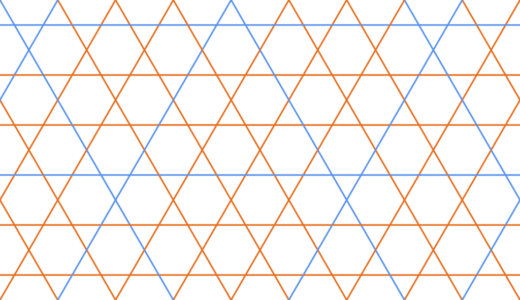
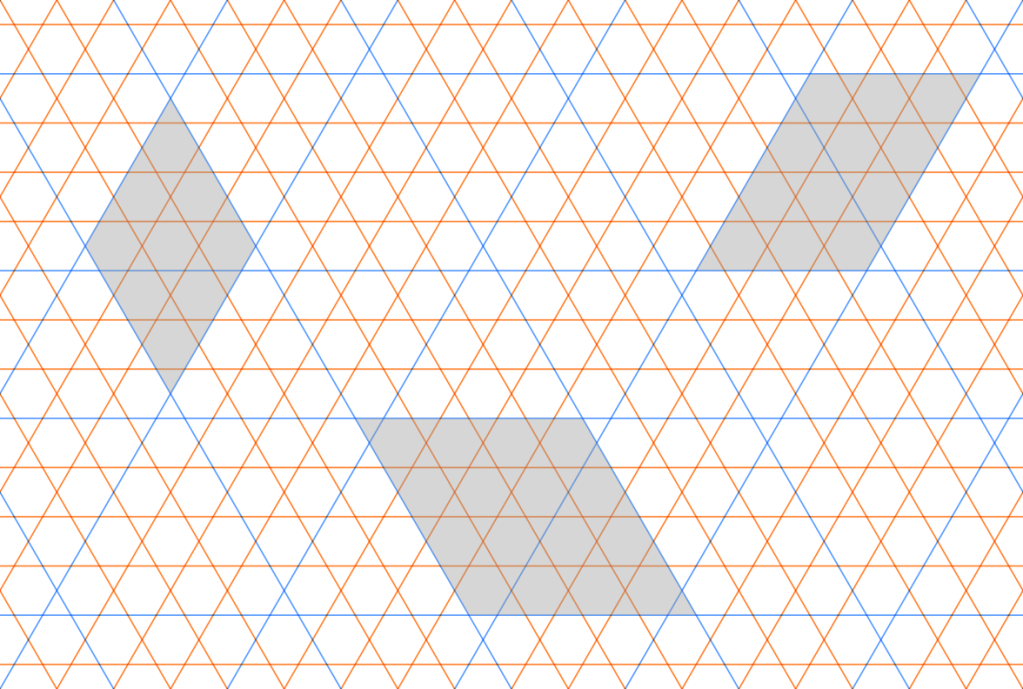
The most important result of the previous post is that every tiling of the plane by Turtle tiles forces a kagome lattice with two line colors to arise. This kagome lattice also exhibits two special properties.

Figure 1: A finite part of an example kagome lattice with two line colours.

The most important of these properties is collation. A two-line-colour Kagome lattice is collated if there is a partition of positive(i.e. same-colour) line crossings into monochrome sets of three, containing one crossing in each orientation forming a ‘smallest’ triangle in the lattice.

The other property was called arationality(formerly irrationality) in the previous post. A two-line-colour kagome lattice is arational if, for every line class(i.e. a maximal set of parallel lines), either the fraction of all lines that are a particular colour is either irrational or not well-defined.

These two properties, for two-colour kagome lattices, are enough to prove the observed ‘evenness’ and how it could be considered maximal.

Class sequences and colour runs

We are interested in the ordering of line colours within a class, so we need some terms to describe this. Let a class sequence be the complete two-sided infinite sequence of line colours in a line class. Let a class ray be a one-sided infinite contiguous part of a class sequence.

Let a factor of a class sequence or ray be a finite string of colours found contiguously in the ray or sequence. Let the set of all a ray’s or sequence’s factors be its factor set. Let an n-factor be a factor with a sequence of n colours. Let a subfactor be a sub-string of a factor, and an extension of a factor be a factor of the parent ray or sequence that has the original factor as a subfactor.

We start where we left off in the previous post with a kagome lattice with our two special properties. Looking at the n-factors, starting at n=1, arationality guarantees that both colours appear in all classes, so each sequence factor set has 2 1-factors.

Let us temporarily denote the two colours as and . Of the four possible 2-factors, arationality guarantees that at least one of or occurs in all of the sequence factor sets. If we try to have both and in the factor sets, then that causes conflicts.

Figure 2: Two line colour doubles in different classes. The dotted line cannot be coloured in without creating an isolated positive crossing. (Other lines not shown)

If and occur in different classes, then that directly conflicts with collation(Figure 2). If and are in the same class, then that forces a periodic alternating pattern in the other two classes, breaking arationality. Thus, exactly one of , can be in any and all factor sets.

Theorem 1: In a two-colour collating and arational kagome lattice, exactly one colour can form doubles or longer single-colour runs.

Let the colour which can come in doubles be the base colour, denoted , and the non-doubling colour be the highlight colour, denoted . Since occurs in all class sequences but there cannot be a before or after it, then and , along with , are the three 2-factors in the class sequence factor sets.

We won’t continue listing off n-factors by length, but the existence of base and highlight lines brings up the question of how long a ‘run’ of base lines in a class can last until it gets ‘capped’ by highlight lines on both ends.

Figure 3: A band(shaded grey) within a kagome lattice.

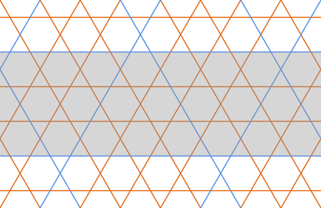
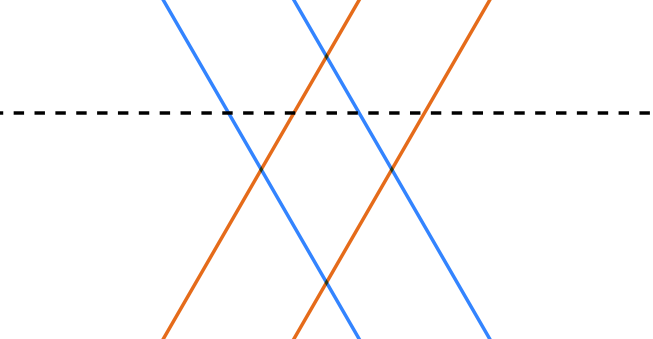
Let a band be an infinite strip of the plane the kagome lattice lies on bounded by parallel highlight lines such that there are no other parallel highlight lines within the band. Let a domain be the parallelogram formed from the intersection of two bands.

Figure 4: Part of a kagome lattice where some domains have been shaded grey.

Every domain has a highlight cutting line completing the collation triangles for its obtuse angles. If the pairs of parallel sides of a domain are too disparate in length, the cutting line strikes the middle of a domain side. By the definition of a domain, this produces an isolated positive crossing, breaking collation(Figure 5).

Figure 5: A ‘overlong’ domain. The cutting line crossing with the bottom side of the domain cannot be put into a collation triangle.

To avoid ‘overlong’ domains, the intersecting bands cannot differ in width by more than one. Since any two bands derived from different line classes will intersect, this restricts band widths in different classes to differ by at most one. This also prevents bands with widths differing by three or more to occur in the same line class.

If two bands occur in the same class with a difference of two, then every band in the other two classes must take the intermediate width, forcing a periodic pattern in those classes and breaking arationality. Converting back to factors and letting be short for a -string of ‘s, we get the following theorems, both of which presuppose a two-colour, arational, collated kagome lattice.

Theorem 2a: If is a factor of some class sequence for some , then exactly one of and is as well.

Theorem 2b: If and are factors in (possibly distinct) class sequences for some positive integer , then in all sequences all factors of the form have or .

To describe it more casually, only -runs or -runs of base lines are allowed to occur and be capped at both ends. Let be the minimum base run length that is capped at both ends, so that and are both factors of all sequences.

Theorems 1, 2a, and 2b are enough to explain the observed even spacing of reflected tiles over small patches of Turtle tilings, but they give us less control over larger scales, as it seems -runs and -runs may occur in arbitrary order. Fortunately, our two special properties can control the order of -runs and -runs to a very strong degree.

Kagome lattices all the way up

Looking for a way to progress further, we note that we started with two line colours in a kagome lattice, and we now have bands that come in two different widths. Like the lines, the bands lie in three classes by parallelism. If there were some way to turn these bands into a kagome lattice, then we may get something.

Figure 6: A kagome lattice of purple lines line and a triangular grid of green dotted lines.

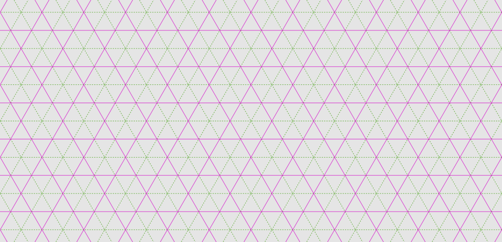
To do that, we need to consider how a kagome lattice can be created. First, we start with a triangular grid(green lines in Fig. 6). Then, we add lines in between the original lines(purple lines in Fig. 6). Both of these lines together produce a triangular grid at half-scale, but the purple lines alone create a kagome lattice.

Figure 7: Two triangular tiles that can be tiled to produce a kagome lattice. The left tile is produced from three decorated kites, while the right tile can produce Fig. 6

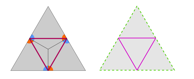
If we break up the lattice and grids in Figure 6 into triangular tiles using the green lines, we get the right triangle in Figure 7. This looks like the tile generated by three decorated kite tiles, from which we first created a kagome lattice.

Looking at an example of a kagome lattice with our special properties in Figure 4, it seems that the highlight lines form something close to a triangular grid. This also make sense when thinking about it, as collation forces highlight lines to meet to form collation triangles, which are much smaller than band widths. Thus, the highlight collation triangles effectively form the vertices of a triangular grid.

Using our idea to create a kagome lattice, each line of the new kagome lattice does correspond to a band, as we had hoped. Theorems 2a and 2b allow us to colour these new ‘lines’ based on corresponding band widths.

While we have a new kagome lattice, we cannot do much with it unless it satisfies our two special properties. First, let us see if arationality holds.

Let be the fraction of all lines in a class that are base lines, and be the fraction that are highlight lines. As then they are rational, irrational, or not well-defined together. Arationality forces , so the fraction is well-defined so long as is. It is also easy to see that goes with and on questions of rationality as well.

Analogously, we can define and as the fraction of bands that are ‘narrow’ and ‘wide’ respectively. Thanks to Theorem 2b, if they are well-defined, and so they also go together on questions of rationality.

To relate these sets of variables, let us consider the contributions of each band width to and . Each narrow band effectively contributes one highlight line and base lines, while wide bands add base lines along with their highlight line. This effectively restricts to the interval , and where it lies in that interval depends on , so we have:

This clearly aligns and with and in terms of well-definedness and rationality, so the arationality property transfers over. Note that even though arationality transfers, the actual values of and do not in general directly transfer to and if they exist.

Figure 8: Part of a kagome lattice where some half-domains have been shaded grey.

We now need to prove that the new kagome lattice is collated. We define a half-domain as the triangle bounded by two sides of a domain next to one acute angle and the cutting line. Any one of the sides of the half-domain can act as a cutting line, so a particular half-domain is ‘part of’ three distinct domains with different orientations. This also implies that every half-domain is at the intersection of three bands. Half-domains are the equivalent of the ‘smallest’ triangles in the new kagome lattice.

Figure 9: A rhombic domain and its bounding lines. The dotted lines indicate where the cutting line may lie.

As we derive line colour in the new kagome lattice from band width, positive crossings correspond to rhombic domains. The cutting line cannot pass symmetrically though the domain, and must bias itself closer to one end of the domain.

Note that, geometrically, our old kagome lattice may not be completely regularly spaced, even if it is combinatorially equivalent to a regularly spaced kagome lattice. Let a ‘unit’ here the part of a line between adjacent crossings, and ‘length’ be a count of those units. The key here is that the non-common lines involved in adjacent crossings are never parallel. This forces an alternation of crossings along a line between the two other classes.

The sides of our rhombic domain are length (small) or (large). When we measure distance between parallel lines, we will do so along lines at 60° instead of perpendicularly for clarity, so we say that two parallel sides of a rhombic domain are or units apart.

Choose an arbitrary rhombic domain, and rotate the entire kagome lattice so that its acute angles lie in a (mostly) vertical line(as shown in Fig. 9) and its cutting line lies below its obtuse angles. This rhombic domain is either a small or large domain.

Figure 10: With K = 2, A large rhombic domain with cutting line below the obtuse angles, and a narrow band above the cutting line. The top band edge crossings with the domain sides break collation.

First suppose that our domain is large. Then, the distance from the cutting line to the top acute angle is . If the band directly above the cutting line were narrow, then the other band edge would strike far below the acute angle, and its crossings with the sides of the domain will be in the middle of them and cannot be collated(Fig.10). Thus, the band above the cutting line is forced to be wide.

On the other hand, the bottom acute angle is units away from the cutting line, so either band with could work there. In either case, the bottom half-domain has side lengths while the top half-domain has side length .

Figure 12: With K = 2, A small rhombic domain with cutting line below the obtuse angles, and a wide band below the cutting line. The lower acute angle of the domain cannot be put into a collation triangle.

For the case of a small rhombic domain, the distance from the cutting line to the bottom acute angle is . If the band directly below the cutting line were wide, the bottom acute angle will end up between base lines and cannot be collated.

The top acute angle is units away from the cutting line, so either band width works with collation. Here the top half-domain has side length while the bottom half-domain has side length .

In each case, exactly one side of a rhombic domain ‘forces’ the band passing through to match width with the domain bands. This creates a triangle whose side length is not . If you look at non-rhombic domains, all of their generated half-domains have side length , so the only way to create ‘extremal'(i.e. side length not equal to ) half-domains is through the ‘forced’ side of a rhombic domain.

As described above, every rhombic domain has one forced side and exactly one extremal half-domain. For any extremal half-domain, any side could act as a cutting line, so each is part of exactly three distinct rhombic domains. This also implies that three equal-width bands converge at the extremal half-domain.

These properties allow extremal half-domains to act as the collation triangles for the new kagome lattice, completing the proof of the following Theorem.

Theorem 3: Given any two-colour, arational, and collated kagome lattice, there exists another two-colour, arational, and collated kagome lattice whose line colours exactly correspond to band widths of the original kagome lattice.

The most important aspect of Theorem 3 is that we can apply it iteratively, so for any applicable kagome lattice, we get an infinite upward stack of kagome lattices generated by repeated applications of Theorem 3.

Note: The stack of kagome lattices produced by Theorem 3 directly from Turtle tiling lattices have no relation to the hierarchical structure of the Turtle tiling. An altered kagome lattice with Theorem 3 may be related to that hierarchy, but that would require more work to justify.

Balanced rays and colour waves

We have obtained an infinite stack of kagome lattices from our original kagome lattice, but what that tells us about the original kagome lattice is obscure.

Let us think about it in terms of Theorems 2a and 2b. When applied to our original kagome lattice, it restricts the lengths of base-line runs between highlight lines, imposing a basic level of ‘evenness’ in the distribution of highlight lines.

Considering Theorems 2a-b on the first kagome lattice up, it applies a restriction on ‘runs of runs’ of base lines, reinforcing highlight line evenness. Theorems 2a-b applied to higher levels of kagome lattices further refine the possible distributions of highlight runs in each class of the original kagome lattice.

In the end, we hope there is some some strong statement that can capture all the stacked ‘evenness’ refinements. Given that each higher level of kagome has a larger effective scale, we expect that such a statement would be global in nature. Luckily, mathematicians have already formulated a property that fulfills our needs and has important consequences.

First, we need to show that our original kagome lattice(in particular, its class sequences) fulfills this property.

Theorem 4: For any string made of the colours and of a two-colour arational collated kagome lattice, at most one of the strings and is a factor in any class sequence.

Proof: First we consider the cases where has at most one colour. The empty string works, as and not is a factor. Strings with only also work, as is the only valid factor that arises from that category of strings.

If a string with only in it fails, that implies that and are both factors, in contradiction to Theorem 2b. Thus, so long as has only one colour, Theorem 4 holds.

Let us now try to construct a string where Theorem 4 fails. Here, in light of Theorems 2a-b, it is best to consider as a separator of ‘blocks’ of and .

For this part we will technically label the colours as and , but we’ll ignore colour subscripts unless new colours and subscripts emerge. Given this, our assumption will be that there is some finite string such that and are both factors.

To comply with Theorems 2a-b, it must be the case that , where consists of blocks of and separated by .

Given our assumption above, is a factor as well. Applying Theorem 3 effectively transforms the separated runs of and into and respectively, while all separators disappear.

Let be the result of this transformation on . The transformations of and are thus and respectively. By Theorem 1, exactly one of and is equal to , with the other equal to .

We now have a situation exactly equivalent to before with , , and . If has only one colour, then at most one of and are factors, contrary to our assumption on . If has two colours, then it is still a strictly shorter string of colours than . Eventually with enough iterations of Theorem 3, there will be some that has only one colour, breaking our assumption.

In the field of combinatorics of words, Theorem 4 grants class sequences a very special property. Theorem 4 along with Proposition 2.1.3. in [3] are sufficient to show that class sequences are balanced, as defined in [3].

It is in this sense that highlight lines, hence ‘flipped’ Turtle tiles, are distributed ‘as evenly as possible’, given the constraints of arationality and collation. Another consequence of this is that and are well-defined and irrational(Corollary 2.1.8. in [3]). Based on results from the previous post, for kagome lattices directly constructed from Turtle tilings, we have:

This also forces the following expression for :

Also, as arationality guarantees aperiodicity of the class sequences and any class rays, Proposition 2.1.13. in [3] shows all class rays are mechanical. The most relevant expression of that fact is the generation of mechanical words by rotation. ‘Unrolling’ the rotation, we get a periodic train of ‘colour waves’.

Figure 13: A set of lines from a single line class laid over a set of colour waves. The width of a blue(h) ribbon is exactly equal to the line spacing, while the overall colour wave period and line spacing are in an irrational ratio. The colour of ribbon a line falls upon determines its own colour.

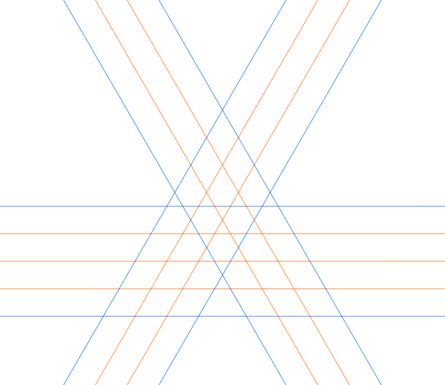
Thus, for every class ray, there exists a colour wave that determines its colour sequence(Figure 13), made up of alternating and ‘ribbons’. All these wave patterns must have -ribbon width equal to the class line spacing, and the ratio of -ribbon to -ribbon widths must be . The only way these waves can differ is in phase.

For all class rays running in the same direction, their waves must be exactly in phase, as if there were any mismatch, the infinitely many shared lines and irrational wave/line period ratio will cause a line to fall into that mismatch. For class rays running in opposed directions, there is at most a finite overlap, but for any given size of phase mismatch, you can choose two class rays with a large enough shared region to guarantee that a line falls into the mismatch. This means that a single colour wave is enough for the entire class sequence, and proves the main result of this post.

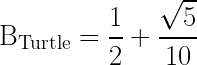
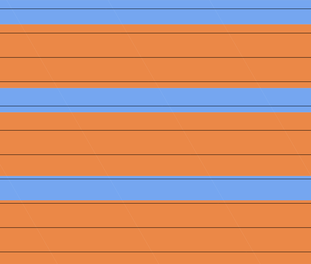
Theorem 5: For any line class of a regularly spaced, two-colour, arational, and collated kagome lattice, there exists a periodic wave pattern of alternating colour ribbons such that for every line in the class lying within a ribbon, its colour matches the colour of the ribbon it lies on. Normalizing the line spacing as , the period of the wave is , with -ribbons of width and -ribbons of width .

Note the addition of the regular spacing constraint that was not present in the previous theorems.

Figure 14: A kagome lattice and its three colour waves, arranged to preserve collation. The colour ribbon widths here are compatible with a Turtle tiling.

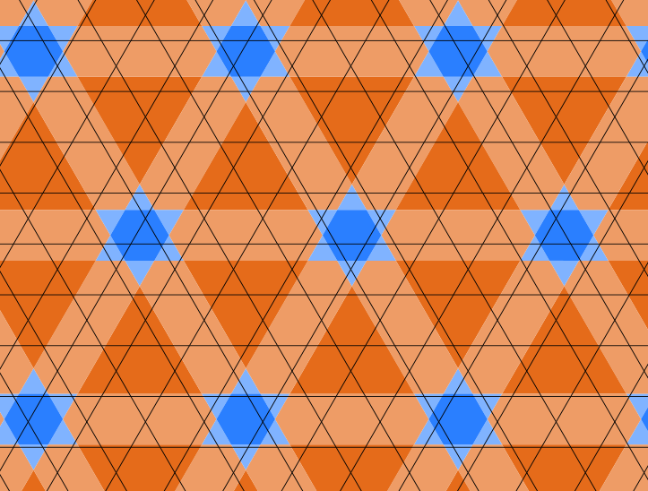
Given the three colour waves Theorem 5 produces, the collation property forces a particular alignment of these waves as shown in Figure 14. Highlight collation triangles, hence flipped Turtle tiles, must occur close to the blue hexagons, but the irrational ratio of periods disrupts exact tile regularity.

Figure 15: A situation where all three classes hit an edge case. The double-ended arrows point to line pairs of which exactly one must be a highlight line.

One special case we need to take care of is when a line lies exactly on a ribbon boundary. Given the width of -ribbons, when this happens, two adjacent lines will lie on the edges of one -ribbon. For any chance of collation holding, exactly one of the edge lines must be a highlight line. For this we can choose a bias direction for each class, whether or not it hits the edge.

If there is only line class hitting the edge, that is sufficient, but in the case of all three classes hitting the edge(Fig. 15), some combinations of bias direction choices fail to protect collation. For this case the bias directions must be asymmetric for collation to hold unconditionally.

Overview and discussion

One way to intuitively see how the the ‘evenness’ of highlight lines arises come from a fact mentioned earlier about how the highlight lines arrange themselves to approximate a triangular grid. Enough ‘irregularities’ in highlight line spacing could disrupt alignment enough to break collation.

What is surprising, however is the ‘stiffness’ of this constraint. In isolation, there are two ways a third highlight line can complete a collation triangle. However, for almost all arational collated kagome lattices, no finite re-arrangement of line colours preserves collation. At best, you can swap the colours of three pairs of parallel adjacent lines.

Some of this surprise likely comes from the abstract and convoluted nature of the proof of Theorem 3, and hence Theorems 4 and 5. A direct proof of the latter two theorems may look like Theorem 3 in Part 1, with witness lines forming functions between line classes. Another observation which may lead to a direct proof concerns the orientation of base collation triangles.

Given two base collation triangles with no highlight lines between them, then they must have the same orientation(point-up or point-down). For every highlight line you cross, the ‘local’ base collation triangles swap orientation.

I haven’t come up with a way to combine these or other observations to produce a more direct proof of Theorem 4 or 5, but I would not be surprised that such a proof existed.

Theorem 5 has significant implications for arrangement of Turtle tiles in their tilings. This will be examined in the next major post.

Reference

[1] Hatfest. “Craig Kaplan – Aperiodic monotiles: new shapes just dropped – Hatfest,” YouTube, Oct 2, 2023, [Video file]. https://www.youtube.com/watch?v=252pJS4U5Zc (accessed Apr. 08, 2024).

[2] D. Smith, J. S. Myers, C. S. Kaplan, and C. Goodman-Strauss, “An aperiodic monotile,” Mar. 2023, doi: https://doi.org/10.48550/arxiv.2303.10798.

[3] M. Lothaire, Algebraic Combinatorics on Words. Cambridge: Cambridge University Press, 2002.